Data Analysis tip - Some new data plotting options!
Derek has developed some plotting routines that let you take a quick look at data without having to extract the data into a file and then utilize a different program (e.g., excel or IDL) to plot it. There is one set of routines that just show you the plot in a window on your computer screen and a second set of routines that save a png of the plot in a directory. The routines are called using either da.show.* or da.plot.*, respectively, where '*' gives the name of the type of plot.
Types of plots available (click on plot thumbnail in table to enlarge)
| da.{type}.timeseries | timeseries plot | |
| da.{type}.allan | Allan noise plot | |
| da.{type}.cdf | Cumulative distribution function plot | |
| da.{type}.cycle | temporal variability box-whisker plot | |
| da.{type}.density | density plot | |
| da.{type}.pdf | probability distribution function plot | |
| da.{type}.scatter | x-y scatter plot |
You have access to these scripts on your aer_vm. To get help with using a plot, type the plots name followed by --help (e.g., da.plot.timeseries --help). This spews out the following:
Time series plot - A two dimensional time series of values.
If used without any data specification (variables, start, etc) then input will be read from standard input. If an existing, readable file is given input will be read from that
file. Otherwise the data given on the command line is read, with the variables determined by the graph's switch(es) if not explicitly specified.
Switches can be given at any point in the command line, however a simple "--" terminates switch processing and all further arguments are treated as bare words.
You can also get help on the arguments to any command, e.g., in the example da.show.timeseries --help=quantile
Arguments:
station The (default) station to read data from
Default: Inferred from the current directory
variables The list of variable specifies to read from the archive
times The time range of data to read
archive The (default) archive to read data from
Default: The "raw" data archive
inputFile The file to read data from or - for standard input
--fit Fit type
Default: Disabled
--grid Grid display
Default: Disabled
--legend Legend display
Default: Inside top left corner
--log Use a logarithmic Y axes
--quantile Filter to the Nth quantile
--title Title
--x-title X axis title
Default: Generated from the axis units.
--y Y Variable
--y-title Y axis title
Default: Generated from the axis units.
--z Z Variable
Examples:
Single trace:
da.show.timeseries --y=BaG_A11 brw A11a 2010:1 2010:2
Or:
da.show.timeseries --y=BaG_A11 file.cpd3
Or:
da.get brw A11a 2010:1 2010:2 | da.show.timeseries --y=BaG_A11
The first two examples only work for stations running cpd3. All our partner stations are running cpd2.
The last command works for cpd2 sites, but 'da.get' needs to be changed to 'data.get'.
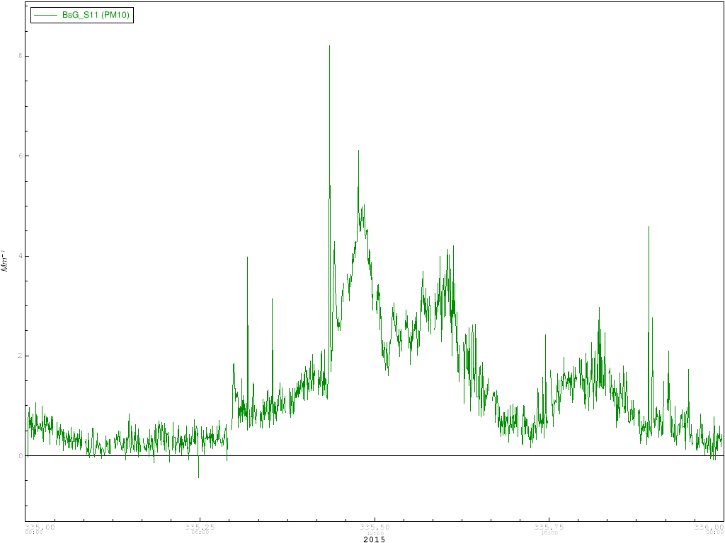
So to plot green scattering at BEO for December 1 2015 you would type:
data.get beo S11a 2015-12-01 2015-12-02 | da.show.timeseries --y=BsG_S11
and the following plot would pop up on your screen:
If instead you typed:
data.get beo S11a 2015-12-01 2015-12-02 | da.plot.timeseries --y=BsG_S11
the plot would be saved to a file (the script defaults to a file called output.png, but you can specify the file name using the switch --file= , e.g., --file=betsys_plot.png)
You can also get help on the arguments to any command, e.g., for the example above:
da.show.timeseries --help=y-title
returns:
This is the title output along the Y axis.
This option takes a single string as a value. For example "--y-title=VALUE"
So you could add an y-title with the following command:
data.get beo S11a 2015-12-01 2015-12-02 | da.show.timeseries --y=BsG_S11 --y-title=scattering
and the following plot would pop up on your screen:
